Study Guide - Limits

Tangent and Velocity Problems

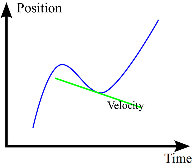
Iinstantaneous velocity can be obtained from a position-time curve of a moving object.

Learning Objectives

Recognize that the slope of a tangent line to a curve gives the instantaneous velocity at that point in time

Key Takeaways

Key Points

Velocity is defined as rate of change of displacement.
The velocity v of the object can be computed as the derivative of position: $\displaystyle \vec{v} = \lim\limits_{\Delta t \to 0}{{\vec{x}(t+\Delta t)-\vec{x}(t)} \over \Delta t}={\mathrm{d} \vec{x} \over \mathrm{d}t}$ .
The equation for an object's position can be obtained by evaluating the integral of the equation for its velocity from time $t_0$ to a later time $t_n$ .

Key Terms

velocity: a vector quantity that denotes the rate of change of position with respect to time, or a speed with the directional component
integral: also sometimes called antiderivative; the limit of the sums computed in a process in which the domain of a function is divided into small subsets and a possibly nominal value of the function on each subset is multiplied by the measure of that subset, all these products then being summed
tangent: a straight line touching a curve at a single point without crossing it there

Calculus has widely used in physics and engineering. In this atom, we will learn that instantaneous velocity can be obtained from a position-time curve of a moving object by calculating derivatives of the curve. Velocity is defined as rate of change of displacement. The average velocity

\bar{\vec{v}}

of an object moving through a displacement (

\Delta \vec{x}

) during a time interval (

\Delta t

) is described by the formula:

\displaystyle \bar{\vec{v}} = \frac{\Delta \vec{x}}{\Delta t}

. What will happen when we reduce the time interval Δt\Delta t and let it approach 0? The average velocity becomes instantaneous velocity at time t. Suppose an object is at positions

\vec{x}(t)

at time

t

and

\vec{x}(t+\Delta t)

time

t + \Delta t

. The velocity

\vec{v}

of the object can be computed as the derivative of position:

\displaystyle \vec{v} = \lim\limits_{\Delta t \to 0}{{\vec{x}(t+\Delta t)-\vec{x}(t)} \over \Delta t}={\mathrm{d} \vec{x} \over \mathrm{d}t}

. Instantaneous velocity is always tangential to trajectory. Slope of tangent of position or displacement time graph is instantaneous velocity and its slope of chord is average velocity.

Instantaneous Velocity: The green line shows the tangential line of the position-time curve at a particular time. Its slope is the velocity at that point.

On the other hand, the equation for an object's position can be obtained mathematically by evaluating the definite integral of the equation for its velocity beginning from some initial period time

t_0

to some point in time later

t_n

. That is

x(t) = x_0 + \int_{t_0}^{t} v(t')~dt'

, where

x_0

is the position of the object at

t=t_0

. For the simple case of constant velocity, the equation gives

x(t)-x_0 = v_0 (t-t_0)

.

Limit of a Function

The limit of a function is a fundamental concept in calculus and analysis concerning the behavior of a function near a particular input.

Learning Objectives

Recognize when a limit does not exist

Key Takeaways

Key Points

The function has a limit $L$ at an input $p$ if $f(x)$ is "close" to $L$ whenever $x$ is "close" to $p$ .
To say that $\displaystyle \lim_{x \to p}f(x) = L$ means that $f(x)$ can be made as close as desired to $L$ by making $x$ close enough, but not equal, to $p$ .
For $x$ approaching $p$ from above (right) and below (left), if both of these limits are equal to $L$ then this can be referred to as the limit of $f(x)$ at $p$ .

Key Terms

secant line: a line that (locally) intersects two points on the curve
function: a relation in which each element of the domain is associated with exactly one element of the co-domain
derivative: a measure of how a function changes as its input changes

The limit of a function is a fundamental concept in calculus and analysis concerning the behavior of that function near a particular input. Informally, a function

f

assigns an output

f(x)

to every input

x

. The function has a limit

L

at an input

p

if

f(x)

is "close" to

L

whenever

x

is "close" to

p

. In other words,

f(x)

becomes closer and closer to

L

as

x

moves closer and closer to

p

. More specifically, when

f

is applied to each input sufficiently close to

p

, the result is an output value that is arbitrarily close to

L

. If the inputs "close" to

p

are taken to values that are very different, the limit is said to not exist. The notion of a limit has many applications in modern calculus. In particular, the many definitions of continuity employ the limit: roughly, a function is continuous if all of its limits agree with the values of the function. It also appears in the definition of the derivative: in the calculus of one variable, this is the limiting value of the slope of secant lines to the graph of a function. To say that

\displaystyle \lim_{x \to p}f(x) = L

means that

f(x)

can be made as close as desired to

L

by making

x

close enough, but not equal, to

p

. Alternatively,

x

may approach

p

from above (right) or below (left), in which case the limits may be written as

\displaystyle \lim_{x \to p^+}f(x) = L_+

or

\displaystyle \lim_{x \to p^-}f(x) = L_-

. If both of these limits are equal to

L

then this can be referred to as the limit of

f(x)

at

p

. Conversely, if they are not both equal to

L

then the limit, as such, does not exist. In the following atoms, we will learn about more strict and precise definition of the limit of a function.

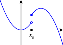
Nonexistence of Limit: The limit as the function approaches $x_0$ from the left does not equal the limit as the function approaches $x_0$ from the right, so the limit of the function at $x_0$ does not exist.

Example: A function without a limit as seen in:

f(x)=\begin{cases}\sin\frac{5}{x-1} & \mbox{ for } x< 1 \\ 0 & \mbox { for } x=1 \\ \frac{0.1}{x-1}& \mbox{ for } x>1\end{cases}

has has no limit at

x_0 = 1

.

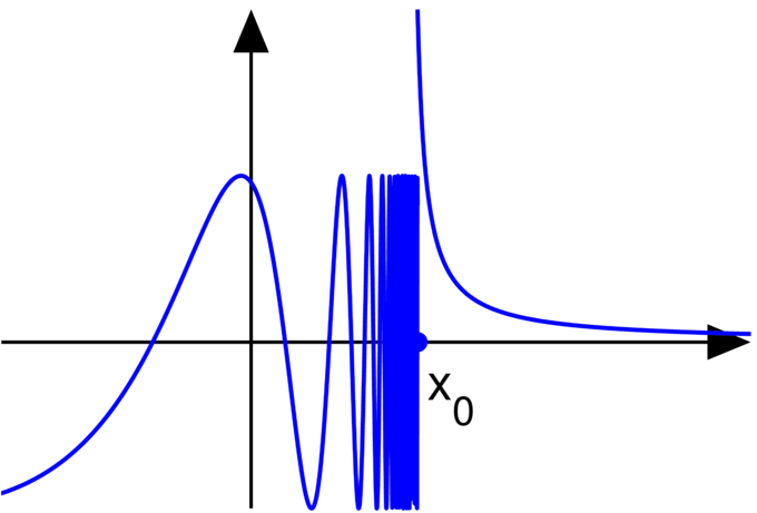
Essential Discontinuity: A graph of the above function, demonstrating that the limit at $x_0$ does not exist.

Calculating Limits Using the Limit Laws

Limits of functions can often be determined using simple laws, such as L'Hôpital's rule and squeeze theorem.

Learning Objectives

Calculate a limit using simple laws, such as L'Hôpital's Rule or the squeeze theorem

Key Takeaways

Key Points

L'Hôpital's rule uses derivatives to help evaluate limits involving indeterminate forms.
When using the L'Hôpital's rule, the differentiation of the numerator and denominator often simplifies the quotient and/or converts it to a determinate form, allowing the limit to be evaluated more easily.
The squeeze theorem is often used to confirm the limit of a function via comparison with two other functions whose limits are known or easily computed.

Key Terms

differentiable: having a derivative, said of a function whose domain and co-domain are manifolds
derivative: a measure of how a function changes as its input changes

Limits of functions can often be determined using simple laws. In this atom, we will study two examples: L'Hôpital's rule or the squeeze theorem.

L'Hôpital's Rule

L'Hôpital's rule (pronounced "lope-ee-tahl," sometimes spelled l'Hospital's rule with silent "s" and identical pronunciation), also called Bernoulli's rule, uses derivatives to help evaluate limits involving indeterminate forms. Application (or repeated application) of the rule often converts an indeterminate form to a determinate form, allowing easy evaluation of the limit. In its simplest form, l'Hôpital's rule states that if functions

f

and

g

are differentiable on an open interval

I

containing

c

, THEN:

$\displaystyle{\lim_{x \to c}f(x)=\lim_{x \to c}g(x)=0 \text{ or } \pm\infty}$
$\displaystyle{\lim_{x\to c}\frac{f'(x)}{g'(x)}}$ exists,
and, if and only if $g'(x)\neq 0 \text{ for all } x \text{ in } I \text{ } (x \neq c)$ , THEN $\displaystyle{\lim_{x\to c}\frac{f(x)}{g(x)} = \lim_{x\to c}\frac{f'(x)}{g'(x)}}$ .

The differentiation of the numerator and denominator often simplifies the quotient and/or converts it to a determinate form, allowing the limit to be evaluated more easily.

The Squeeze Theorem

The squeeze theorem is a technical result that is very important in proofs in calculus and mathematical analysis. It is typically used to confirm the limit of a function via comparison with two other functions whose limits are known or easily computed. The squeeze theorem is formally stated as follows: Let

I

be an interval having the point

a

as a limit point. Let

f

,

g

, and

h

be functions defined on

I

, except possibly at

a

itself. Suppose that for every

x

in

I

not equal to

a

, we have

g(x) \leq f(x) \leq h(x)

, and also suppose that

\lim_{x \to a} g(x) = \lim_{x \to a} h(x) = L

, then

\lim_{x \to a} f(x) = L

.

Squeeze Theorem: $x^2 sin \left ( \frac{1}{x} \right)$ being squeezed by $x^2$ and $-x^2$ in the limit as $x$ approaches $0$ .

Precise Definition of a Limit

The

(\varepsilon,\delta)

-definition of limit (the "epsilon-delta definition") is a formalization of the notion of limit.

Learning Objectives

Explain the meaning of

\delta

in the

(\varepsilon,\delta)

-definition of a limit.

Key Takeaways

Key Points

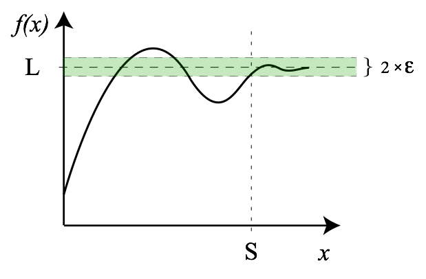
Suppose $f:R \rightarrow R$ is defined on the real line and $p,L \in R$ . It is said the limit of $f$ as $x$ approaches $p$ is $L$ and written $lim_{x} \rightarrow pf(x)=L\lim_{x \to p}f(x) = L$ , if the following property holds. (Continued).
For every real $\varepsilon > 0$ , there exists a real $\delta > 0$ such that for all real $x$ , $\varepsilon > 0$ $0 < \left | x-p \right | < \delta$ implies $\left | f(x) - L \right | < \varepsilon$ . Note that the value of the limit does not depend on the value of $f(p)$ , nor even that $p$ be in the domain of $f$ .
This definition also works for functions with more than one input value.

Key Terms

infinity: a number that has an infinite numerical value that cannot be counted
error: the difference between a measured or calculated value and a true one

The

(\varepsilon,\delta)

-definition of limit ("epsilon-delta definition of limit") is a formalization of the notion of limit. It was first given by Bernard Bolzano in 1817, followed by a less precise form by Augustin-Louis Cauchy. The definitive modern statement was ultimately provided by Karl Weierstrass.

The $(\varepsilon,\delta)$ -Definition

The

(\varepsilon,\delta)

-definition of limit is a formalization of the notion of limit. Suppose

f:R \rightarrow R

is defined on the real line and

p,L \in R

. It is said the limit of

f

as

x

approaches

p

is

L

and written

lim_{x} \rightarrow pf(x)=L\lim_{x \to p}f(x) = L

, if the following property holds:

For every real $\varepsilon > 0$ , there exists a real $\delta > 0$ such that for all real $x$ , $\varepsilon > 0$ $0 < \left | x-p \right | < \delta$ implies $\left | f(x) - L \right | < \varepsilon$ . Note that the value of the limit does not depend on the value of $f(p)$ , nor even that $p$ be in the domain of $f$ .

Definitely of a Limit: Whenever a point $x$ is within $\delta$ units of $c$ , $f(x)$ is within $\epsilon$ units of $L$ .

Example

For an arbitrarily small

\varepsilon

, there always exists a large enough number

N

such that when

x

approaches

N

,

\left | f(x)-L \right | < \varepsilon

. Therefore, the limit of this function at infinity exists.

Limit of a Function at Infinity: For an arbitrarily small $\epsilon$ , there always exists a large enough number $N$ such that when $x$ approaches $N$ , $\left | f(x)-L \right | < \varepsilon$ . Therefore, the limit of this function at infinity exists.

The letters

\varepsilon

and

\delta

can be understood as " error " and "distance," and in fact Cauchy used

\epsilon

as an abbreviation for "error" in some of his work. In these terms, the error

(\varepsilon)

in the measurement of the value at the limit can be made as small as desired by reducing the distance

(\delta)

to the limit point. This definition also works for functions with more than one input value. In those cases,

\delta

can be understood as the radius of a circle or sphere or higher-dimensional analogy, in the domain of the function and centered at the point where the existence of a limit is being proven, for which every point inside produces a function value less than ε from the value of the function at the limit point.

Continuity

A continuous function is a function for which, intuitively, "small" changes in the input result in "small" changes in the output.

Learning Objectives

Distinguish between continuous and discontinuous functions

Key Takeaways

Key Points

If a function is not continuous, it is said to be a "discontinuous function."
The function $f$ is continuous at some point $c$ of its domain if the limit of $f(x)$ as $x$ approaches $c$ through the domain of $f$ exists and is equal to $f(c)$ .
The function $f$ is said to be continuous if it is continuous at every point of its domain.

Key Terms

bicontinuous: homomorphic or of structure-preserving mapping
topology: a branch of mathematics studying those properties of a geometric figure or solid that are not changed by stretching, bending and similar homeomorphisms

A continuous function is a function for which, intuitively, "small" changes in the input result in "small" changes in the output. Otherwise, a function is said to be a "discontinuous function." A continuous function with a continuous inverse function is called "bicontinuous." Continuity of functions is one of the core concepts of topology. Example: Consider the function

h(t)

, which describes the height of a growing flower at time

t

. This function is continuous. In fact, a dictum of classical physics states that in nature everything is continuous. By contrast, if

M(t)

denotes the amount of money in a bank account at time

t

, then the function jumps whenever money is deposited or withdrawn, so the function

M(t)

is discontinuous. The function

f

is continuous at some point

c

of its domain if the limit of

f(x)

as

x

approaches

c

through the domain of

f

exists and is equal to

f(c)

. In mathematical notation, this is written as

\lim_{x \to c}{f(x)} = f(c)

. In detail this means three conditions:

$f$ has to be defined at $c$ ,
the limit on the left-hand side of that equation has to exist, and
the value of this limit must equal $f(c)$ .

The function

f

is said to be continuous if it is continuous at every point of its domain. If the point

c

in the domain of

f

is not a limit point of the domain, then this condition is vacuously true, since

x

cannot approach

c

through values not equal to

c

.

Finding Limits Algebraically

For a real-valued function expressed in terms of other functions, limit values may be computed via algebraic operations.

Learning Objectives

Compute limit values algebraically using properties of limits

Key Takeaways

Key Points

Algebraic limit theorem states that $\begin{matrix} \lim\limits_{x \to p} & (f(x) + g(x)) & = & \lim\limits_{x \to p} f(x) + \lim\limits_{x \to p} g(x) \\ \lim\limits_{x \to p} & (f(x) - g(x)) & = & \lim\limits_{x \to p} f(x) - \lim\limits_{x \to p} g(x) \\ \lim\limits_{x \to p} & (f(x)\cdot g(x)) & = & \lim\limits_{x \to p} f(x) \cdot \lim\limits_{x \to p} g(x) \\ \lim\limits_{x \to p} & (f(x)/g(x)) & = & {\lim\limits_{x \to p} f(x) / \lim\limits_{x \to p} g(x)} \end{matrix}$ .
In each case above, when the limits on the right do not exist, nonetheless the limit on the left, called an indeterminate form, may still exist.
When algebraic limit theorem doesn't yield a limit value, corresponding limits might often be determined with L'Hôpital's rule or the Squeeze theorem.

Key Terms

limit: a value to which a sequence or function converges
algebraic: containing only numbers, letters, and arithmetic operators

If

f

is a real-valued (or complex-valued) function, then taking the limit is compatible with the algebraic operations, provided the limits on the right sides of the equations below exist (the last identity holds only if the denominator is non-zero). This set of rules is often called the algebraic limit theorem, expressed formally as follows:

\displaystyle{\begin{matrix} \lim\limits_{x \to p} & (f(x) + g(x)) & = & \lim\limits_{x \to p} f(x) + \lim\limits_{x \to p} g(x) \\ \lim\limits_{x \to p} & (f(x) - g(x)) & = & \lim\limits_{x \to p} f(x) - \lim\limits_{x \to p} g(x) \\ \lim\limits_{x \to p} & (f(x)\cdot g(x)) & = & \lim\limits_{x \to p} f(x) \cdot \lim\limits_{x \to p} g(x) \\ \lim\limits_{x \to p} & \left ( \frac{f(x)}{g(x)} \right ) & = & \frac{\lim\limits_{x \to p} f(x)} {\lim\limits_{x \to p} g(x)} \end{matrix}}

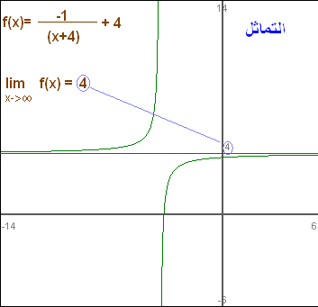
Finding a Limit: The limit of $f(x)= \frac{-1}{(x+4)} + 4$ as $x$ goes to infinity can be segmented down into two parts: the limit of $\frac{−1}{(x+4)}$ and the limit of $4$ . The former is $0$ , while the latter is $4$ . Therefore, the limit of $f(x)$ as $x$ goes to infinity is $4$ .

In each case above, when the limits on the right do not exist (or, in the last case, when the limits in both the numerator and the denominator are zero), the limit on the left, called an indeterminate form, may nonetheless still exist—this depends on the functions f and g. These rules are also valid for one-sided limits, for the case

p = \pm

, and also for infinite limits using the following rules:

\displaystyle{\begin{matrix} &q + \infty &=& \infty \text{ for } q \neq - \infty \\ &q \cdot \infty &=& \infty \text{ if } q > 0 \\ &q \cdot \infty &=& -\infty \text{ if } q < 0 \\& \frac{q}{\infty} &=& 0 \text{ if } q \neq \pm \infty \end{matrix}}

Note that there is no general rule for the case

\frac{q}{0}

; it all depends on the way

0

is approached. Indeterminate forms—for instance,

\frac{0}{0}

,

0 \cdot

some number,

\infty

, and

\frac{\infty}{\infty}

are also not covered by these rules, but the corresponding limits can often be determined with L'Hôpital's rule or the squeeze theorem. We will study these rules in the following atoms.

Trigonometric Limits

There are several limits of special interest involving trigonometric functions.

Learning Objectives

Identify the limits of special interest involving trigonometric functions

Key Takeaways

Key Points

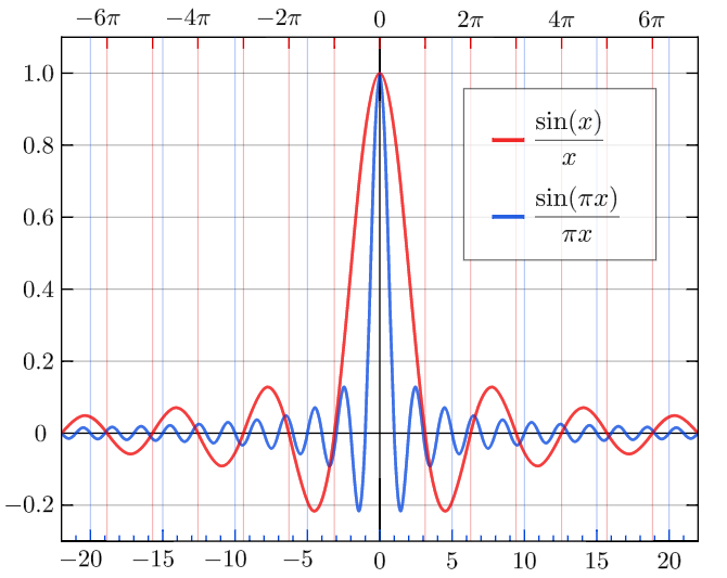
The limit $\lim_{x \to 0} \frac{\sin x}{x} = 1$ is the most important relation involving limits of trigonometric functions.
Using the first relation, we can also get $\lim_{x \to 0} \frac{1 - \cos x}{x} = 0$ .
By substituting $t=\frac{1}{x}$ in the first relation, we get $\lim_{x \rightarrow \infty} x \sin \left (\frac{c}{x} \right ) = c$ .

Key Terms

squeeze theorem: theorem obtaining the limit of a function via comparison with two other functions whose limits are known or easily computed
trigonometric function: any function of an angle expressed as the ratio of two of the sides of a right triangle that has that angle, or various other functions that subtract 1 from this value or subtract this value from 1 (such as the versed sine)

There are several limits of special interest involving trigonometric functions.

1. $\displaystyle{\lim_{x \to 0} \frac{\sin x}{x} = 1}$

This limit can be proven with the squeeze theorem. For

0 < x < \frac{ \pi}{2}

,

\sin x < x < \tan x.

Dividing everything by

\sin x

yields:

1 < \frac{x}{\sin x} < \frac{\tan x}{\sin x}

which reduces to:

\displaystyle{1 < \frac{x}{\sin x} < \frac{1}{\cos x}}

. Taking the limit of the right-hand side:

\displaystyle{\lim_{x \to 0} \left ( \frac{1}{\cos x} \right ) = \frac{1}{1} = 1}

The squeeze theorem tells us that:

\displaystyle{\lim_{x \to 0} \left ( \frac{x}{\sin x} \right ) = 1}

Equivalently:

\displaystyle{\lim_{x \to 0} \left ( \frac{\sin x}{x} \right ) = 1}

Sinc Function: The normalized sinc (blue, higher frequency) and unnormalized sinc function (red, lower frequency) shown on the same scale.

2. $\displaystyle{\lim_{x \to 0} \frac{1 - \cos x}{x} = 0}$

This equation can be proven with the first limit and the trigonometric identity

1 - \cos^2 x = \sin^2 x

. We start with:

\displaystyle{\frac{1 - \cos x}{x}}

Multiplying the numerator and denominator by

1 + \cos x

,

\displaystyle{\frac{(1−\cos x)(1+\cos x)}{x(1+\cos x)}=\frac{(1−\cos^2x)}{x(1+\cos x)}=\frac{\sin^2x}{x(1+\cos x)}= \frac{\sin x}{x} \cdot \frac{\sin x}{1+\cos x}}

Using the algebraic limit theorem,

\displaystyle{\lim_{x \to 0}\left ( \frac{\sin x}{x} \frac{\sin x}{1 + \cos x} \right ) = \left (\lim_{x \to 0} \frac{\sin x}{x} \right ) \left ( \lim_{x \to 0} \frac{\sin x}{1 + \cos x} \right ) = \left (1 \right )\left (\frac{0}{2} \right )= 0}

Therefore:

\displaystyle{\lim_{x \to 0} \frac{1 - \cos x}{x} = 0}

3. $\lim_{x \to \infty} x \sin \left(\frac{c}{x}\right) = c$

This relation can be proven by substituting

t=\frac{1}{x}

into the first relation we derived:

\displaystyle{\lim_{t \to 0} \left ( \frac{\sin t}{t} \right ) = 1}

.

Intermediate Value Theorem

For a real-valued continuous function

f

on the interval

[a,b]

and a number

u

between

f(a)

and

f(b)

, there is a

c \in [a,b]

such that

f(c)=u

.

Learning Objectives

Use the intermediate value theorem to determine whether a point exists on a continuous function

Key Takeaways

Key Points

The intermediate value theorem states that for each value between the least upper bound and greatest lower bound of the image of a continuous function there is at least one point in its domain that the function maps to that value.
The theorem is frequently stated in the following equivalent form: Suppose that $f: [a, b] \to R$ is continuous and that $u$ is a real number satisfying $f(a) < u < f(b)$ or $f(a) > u > f(b)$ . Then for some $c \in [a, b]$ , $f(c) = u$ .
The theorem depends on (and is actually equivalent to) the completeness of the real numbers.

Key Terms

real number: a value that represents a quantity along a continuous line
completeness of the real numbers: completeness implies that there are not any "gaps" or "missing points" in the real number line
continuous function: a function whose value changes only slightly when its input changes slightly

The intermediate value theorem states that for each value between the least upper bound and greatest lower bound of the image of a continuous function there is at least one point in its domain that the function maps to that value. There are three ways of stating the intermediate value theorem:

Version I: If $f$ is a real-valued continuous function on the interval $[a, b]$ , and $u$ is a number between $f(a)$ and $f(b)$ , then there is a $c \in [a, b]$ such that $f(c) = u$ .
Version 2: Suppose that $f: [a, b] \to R$ is continuous and that u is a real number satisfying $f(a) < u < f(b)$ or $f(a) > u > f(b)$ . Then for some $c \in [a, b]$ , $f(c) = u$ .
Version 3: Suppose that $I$ is an interval $[a, b]$ in the real numbers $\mathbb{R}$ and that $f: I \to R$ is a continuous function. Then the image set $f(I)$ is also an interval, and either it contains $[f(a), f(b)]$ , or it contains $[f(b), f(a)]$ ; that is, $f(I) \supseteq [f(a), f(b)]$ , or $f(I) \supseteq [f(b), f(a)]$ .

This captures an intuitive property of continuous functions: given

f

continuous on

[1, 2]

, if

f(1) = 3

and

f(2) = 5

, then

f

must take the value

4

somewhere between

1

and

2

. It represents the idea that the graph of a continuous function on a closed interval can be drawn without lifting your pencil from the paper. The theorem depends on (and is actually equivalent to) the completeness of the real numbers. It is false for the rational numbers

\mathbb{Q}

. For example, the function

f(x) = x^2 − 2

for

x \in \mathbb{Q}

satisfies

f(0) = −2

and

f(2) = 2

. However there is no rational number

x

such that

f(x) =0

, because

\sqrt 2

is irrational. The intermediate value theorem can be used to show that a polynomial has a solution. For example,

x^2-1

. The IVT shows that this has at least one point where

x=0

because at

x=0

it is negative and at

x=2

it is positive. Therefore, since it is continuous, there must be at least one point where

x

is

0

.

Infinite Limits

Limits involving infinity can be formally defined using a slight variation of the

(\varepsilon, \delta)

-definition.

Learning Objectives

Evaluate the limits of functions as

x

approaches infinity

Key Takeaways

Key Points

For $f(x)$ a real function, the limit of $f$ as $x$ approaches infinity is $L$ , means that for all ε>0\varepsilon > 0, there exists $c$ such that whenever $x > c$ , |f(x)−L|<ε|f(x) - L| < \varepsilon.
For a rational function $f(x)$ of the form $\frac{p(x)}{q(x)}$ , there are three basic rules for evaluating limits at infinity, where $p(x)$ and $q(x)$ are polynomials.
If the limit at infinity exists, it represents a horizontal asymptote at $y = L$ .

Key Terms

definition: a formalization of the notion of the limit of functions
asymptote: a straight line which a curve approaches arbitrarily closely, as they go to infinity

Limits involving infinity can be formally defined using a slight variation of the

(\varepsilon, \delta)

-definition. For

f(x)

a real function, the limit of

f

as

x

approaches infinity is

L

, denoted

\lim_{x \to \infty}f(x) = L

, means that for all

\varepsilon > 0

, there exists

c

such that

\left | f(x) - L \right | < \varepsilon

whenever

x>c

. Or, formally:

\forall \varepsilon > 0 \; \exists c \; \forall x < c:\; \left | f(x) - L \right | < \varepsilon

Infinite Limit: For any arbitrarily small $\varepsilon$ , there exists a large enough $N$ such that when $x > N$ , $\left | f(x)-2 \right | < \varepsilon$ . Therefore, the limit of this function at infinity exists.

Similarly, the limit of

f

as

x

approaches negative infinity is

L

, denoted

\lim_{x \to -\infty}f(x) = L

, means that for all

\varepsilon > 0

there exists

c

such that

|f(x) - L| < \varepsilon

whenever

x<c

. For a rational function

f(x)

of the form

\frac{p(x)}{q(x)}

, there are three basic rules for evaluating limits at infinity (

p(x)

and

q(x)

are polynomials):

If the degree of $p$ is greater than the degree of $q$ , then the limit is positive or negative infinity depending on the signs of the leading coefficients;
If the degree of $p$ and $q$ are equal, the limit is the leading coefficient of $p$ divided by the leading coefficient of $q$ ;
If the degree of $p$ is less than the degree of $q$ , the limit is $0$ .

If the limit at infinity exists, it represents a horizontal asymptote at

y = L

. Polynomials do not have horizontal asymptotes; such asymptotes may however occur with rational functions.

Guias de estudo > Boundless Calculus

Limits

Tangent and Velocity Problems

Learning Objectives

Key Takeaways

Key Points

Key Terms

Limit of a Function

Learning Objectives

Key Takeaways

Key Points

Key Terms

Calculating Limits Using the Limit Laws

Learning Objectives

Key Takeaways

Key Points

Key Terms

L'Hôpital's Rule

The Squeeze Theorem

Precise Definition of a Limit

Learning Objectives

Key Takeaways

Key Points

Key Terms

The (ε,δ)(\varepsilon,\delta)(ε,δ)-Definition

Example

Continuity

Learning Objectives

Key Takeaways

Key Points

Key Terms

Finding Limits Algebraically

Learning Objectives

Key Takeaways

Key Points

Key Terms

Trigonometric Limits

Learning Objectives

Key Takeaways

Key Points

Key Terms

1. lim⁡x→0sin⁡xx=1\displaystyle{\lim_{x \to 0} \frac{\sin x}{x} = 1}x→0lim​xsinx​=1

2. lim⁡x→01−cos⁡xx=0\displaystyle{\lim_{x \to 0} \frac{1 - \cos x}{x} = 0}x→0lim​x1−cosx​=0

3. lim⁡x→∞xsin⁡(cx)=c\lim_{x \to \infty} x \sin \left(\frac{c}{x}\right) = climx→∞​xsin(xc​)=c

Intermediate Value Theorem

Learning Objectives

Key Takeaways

Key Points

Key Terms

Infinite Limits

Learning Objectives

Key Takeaways

Key Points

Key Terms

Licenses & Attributions

CC licensed content, Shared previously

CC licensed content, Specific attribution

The $(\varepsilon,\delta)$ -Definition

1. $\displaystyle{\lim_{x \to 0} \frac{\sin x}{x} = 1}$

2. $\displaystyle{\lim_{x \to 0} \frac{1 - \cos x}{x} = 0}$

3. $\lim_{x \to \infty} x \sin \left(\frac{c}{x}\right) = c$